【计算机视觉】pydensecrf在灰度图上的使用
pydensecrf 安装
直接 pip install git+https://github.com/lucasb-eyer/pydensecrf.git 即可安装
对于灰度图的使用 addPairwiseBilateral 不 work
典型的RGB图像设置二元势函数的方式
    d.addPairwiseGaussian(sxy=20, compat=3)
    d.addPairwiseBilateral(sxy=30, srgb=20, rgbim=img, compat=10)
对于GrayScale的图像,无法使用该函数进行调用,而应该使用下面的方式进行调用设置:
pairwise_energy = create_pairwise_bilateral(sdims=(10,10), schan=(0.01,), img=img, chdim=2)
d.addPairwiseEnergy(pairwise_energy, compat=10)  # `compat` is the "strength" of this potential.
下面进行详细介绍:
定义使用一元势函数
一元势函数指的就是分割后得到的class-probabilities,比如来自random-forest或者深度网络的softmax输出。
import pydensecrf.densecrf as dcrf
from pydensecrf.utils import unary_from_softmax, create_pairwise_bilateral
import numpy as np
import matplotlib.pyplot as plt
from scipy.stats import multivariate_normal
plt.rcParams['image.interpolation'] = 'nearest'
plt.rcParams['image.cmap'] = 'gray'
H, W, NLABELS = 400, 512, 2
# This creates a gaussian blob...
pos = np.stack(np.mgrid[0:H, 0:W], axis=2)
rv = multivariate_normal([H//2, W//2], (H//4)*(W//4))
probs = rv.pdf(pos)
# ...which we project into the range [0.4, 0.6]
probs = (probs-probs.min()) / (probs.max()-probs.min())
probs = 0.5 + 0.2 * (probs-0.5)
# The first dimension needs to be equal to the number of classes.
# Let's have one "foreground" and one "background" class.
# So replicate the gaussian blob but invert it to create the probability
# of the "background" class to be the opposite of "foreground".
probs = np.tile(probs[np.newaxis,:,:],(2,1,1))
probs[1,:,:] = 1 - probs[0,:,:]
# Let's have a look:
plt.figure(figsize=(15,5))
plt.subplot(1,2,1); plt.imshow(probs[0,:,:]); plt.title('Foreground probability'); plt.axis('off'); plt.colorbar();
plt.subplot(1,2,2); plt.imshow(probs[1,:,:]); plt.title('Background probability'); plt.axis('off'); plt.colorbar();
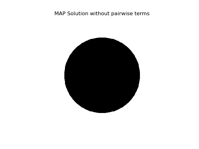
# 有了一元势函数即可开展对应的推理
# Inference without pair-wise terms
U = unary_from_softmax(probs) # note: num classes is first dim
d = dcrf.DenseCRF2D(W, H, NLABELS)
d.setUnaryEnergy(U)
# Run inference for 10 iterations
Q_unary = d.inference(10)
# The Q is now the approximate posterior, we can get a MAP estimate using argmax.
map_soln_unary = np.argmax(Q_unary, axis=0)
# Unfortunately, the DenseCRF flattens everything, so get it back into picture form.
map_soln_unary = map_soln_unary.reshape((H,W))
# And let's have a look.
plt.imshow(map_soln_unary); plt.axis('off'); plt.title('MAP Solution without pairwise terms');

定义使用二元势函数
这个就是要使用到像素之间(包括像素位置以及像素大小)的关系来对预测结果进行平滑。一般使用的就是双边滤波对应的二元势函数。空间以及像素灰度级,对于彩色图来讲一般是xyrgb五个维度,而对于灰度图可能只有xyi三个维度。双边滤波对应的二元势函数描述的就是像素是否是颜色相似或者位置相似,从而可能是属于相同的类别。
下面直接定义一个单通道的灰度图用来让双边滤波进行参考,记住通道为最后一维度:
NCHAN=1

# Create simple image which will serve as bilateral.
# Note that we put the channel dimension last here,
# but we could also have it be the first dimension and
# just change the `chdim` parameter to `0` further down.
img = np.zeros((H,W,NCHAN), np.uint8)
img[H//3:2*H//3,W//4:3*W//4,:] = 1

plt.imshow(img[:,:,0]); plt.title('Bilateral image'); plt.axis('off'); plt.colorbar();

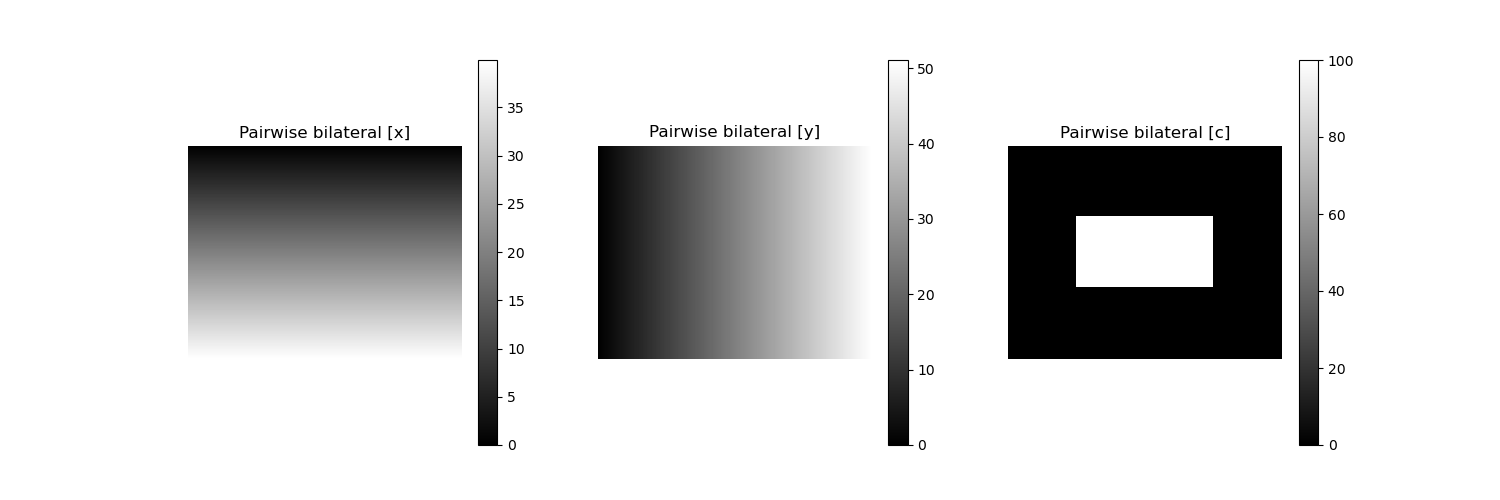
紧接着用上面创建的图像创建二元势函数。
# Create the pairwise bilateral term from the above image.
# The two `s{dims,chan}` parameters are model hyper-parameters defining
# the strength of the location and image content bilaterals, respectively.
pairwise_energy = create_pairwise_bilateral(sdims=(10,10), schan=(0.01,), img=img, chdim=2)

# pairwise_energy now contains as many dimensions as the DenseCRF has features,
# which in this case is 3: (x,y,channel1)
img_en = pairwise_energy.reshape((-1, H, W))  # Reshape just for plotting
plt.figure(figsize=(15,5))
plt.subplot(1,3,1); plt.imshow(img_en[0]); plt.title('Pairwise bilateral [x]'); plt.axis('off'); plt.colorbar();
plt.subplot(1,3,2); plt.imshow(img_en[1]); plt.title('Pairwise bilateral [y]'); plt.axis('off'); plt.colorbar();
plt.subplot(1,3,3); plt.imshow(img_en[2]); plt.title('Pairwise bilateral [c]'); plt.axis('off'); plt.colorbar();
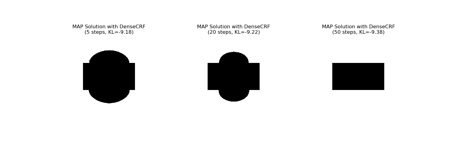
最后一步就是进行完整的DenseCRF推理:
d = dcrf.DenseCRF2D(W, H, NLABELS)
d.setUnaryEnergy(U)
d.addPairwiseEnergy(pairwise_energy, compat=10)  # `compat` is the "strength" of this potential.

# This time, let's do inference in steps ourselves
# so that we can look at intermediate solutions
# as well as monitor KL-divergence, which indicates
# how well we have converged.
# PyDenseCRF also requires us to keep track of two
# temporary buffers it needs for computations.
Q, tmp1, tmp2 = d.startInference()
for _ in range(5):
    d.stepInference(Q, tmp1, tmp2)
kl1 = d.klDivergence(Q) / (H*W)
map_soln1 = np.argmax(Q, axis=0).reshape((H,W))

for _ in range(20):
    d.stepInference(Q, tmp1, tmp2)
kl2 = d.klDivergence(Q) / (H*W)
map_soln2 = np.argmax(Q, axis=0).reshape((H,W))

for _ in range(50):
    d.stepInference(Q, tmp1, tmp2)
kl3 = d.klDivergence(Q) / (H*W)
map_soln3 = np.argmax(Q, axis=0).reshape((H,W))

img_en = pairwise_energy.reshape((-1, H, W))  # Reshape just for plotting
plt.figure(figsize=(15,5))
plt.subplot(1,3,1); plt.imshow(map_soln1);
plt.title('MAP Solution with DenseCRF\n(5 steps, KL={:.2f})'.format(kl1)); plt.axis('off');
plt.subplot(1,3,2); plt.imshow(map_soln2);
plt.title('MAP Solution with DenseCRF\n(20 steps, KL={:.2f})'.format(kl2)); plt.axis('off');
plt.subplot(1,3,3); plt.imshow(map_soln3);
plt.title('MAP Solution with DenseCRF\n(75 steps, KL={:.2f})'.format(kl3)); plt.axis('off');
2020-04-10